Tips of Drafting an R Markdown Document

When presenting the data summary and exploratory analysis, we used to copy a lot of tables, charts from Rstudio to PowerPoint, which makes the presentation preparation painful. It becomes essential for data scientists to make use of better reporting tools, such as R markdown, Jupyter notebook to prepare the analysis presentation in a more efficient and organized way. Of course, we want this to be reproducible!

In this post, I would like to share some tips of using the right tools to draw tables, plot charts, summarize datasets, when I explore building report using R markdown/notebook.

Configuring the notebook

The configure of notebook is set by the YAML header at the beginning of the Rmd file.

• title: the title of the document
• author: name of the author, the email address within the <> will be displayed as a link
• date: can be static or inline R code to reflect modified date.
• output: the rendering options. If set to html_notebook, an HTML file ended with nb.html will be automatically generated whenever the Rmd file is saved. Some other options are also available (i.e. html_document, word_document, pdf_document), if we are going produce other formats of documents.

The following YAML header serves as a good template. The options are commented for easy explanation. The detail of the output options can be found in R Markdown: The Definitive Guide html document section.

---
title: "Tips of Drafting an R markdown document"
author: "Chaoran Liu <6chaoran@gmail.com>"
date: "`r Sys.Date()`"    # can be static "2020-10-25" or "`r Sys.Date()`"
output: 
  html_notebook:
    code_folding: hide    # hide / show, default option for the code display
    theme: default        # the Bootstrap theme to use for the page
    highlight: kate       # R code highighter
    toc_depth: 2          # how deep should the table of content be visible
    toc_float:            # a float toc will stick to the sidebar when scrolling
      collapsed: false
    number_sections: yes  # whether add number index before section header
---

Choosing the theme

The default themes are drawn from Bootswatch library and can be previewed from here. Although there are a variety of themes, they still look quite primitive.

For a more appealing look, I found rmdformats package provides an alternative to the default theme by replacing the output options with the following.

output: 
  rmdformats::readthedown:
    code_folding: hide
    highlight: kate
    number_sections: yes
---

the following screenshot is an example of rendered document from rmdformats::readthedown, of course the package rmdformats need to be installed before hand.

Customizing with CSS

If you are familiar with some basic CSS, you can further tune the formats as you wish. For example, I’m not happy with the header color and the narrow body section of the rmdformats::readthedown theme, I just need to add a css section in the Rmd file.

  #content {
    max-width: 1400px;
  }
  #sidebar h2 {
    background-color: #008B8B;
  }
  h1, h2 {
    color: #008B8B;
  }

Notebook Global Setup

When we’ve done the notebook configuration, theme and format customization, we are good to start drafting our R notebook. The very first R code chunk should be named setup, which can be used to declare global variables, settings and load all used libaries.

In the following example, I hindered the warning and message printing and set the all plots size to be 12 * 6.

knitr::opts_chunk$set(
  warning = FALSE,
  message = FALSE,
  fig.width = 12,
  fig.height = 6
)
library(dplyr)
library(data.table)
library(knitr)
library(kableExtra)
library(DT)
library(ggplot2)
library(plotly)
library(ggpubr)
library(echarts4r)
library(googleVis)

Drafting the document

The Rmarkdown code can be lengthy when we are writing a comprehensive EDA report. There are some tips may help you with your markdown document authoring.

1. list the section headers to construct the document layout, so that you can quickly navigate to the sections
2. put placeholders, such as [TODO] for later modification
3. avoid hard-coded numbers, using inline r code to parameterize the number reporting
4. separate the data processing and document rendering in R script and Rmd file. It can make the report drafting and rendering more productive, because it doesn't require re-generating the intermediate R objects everytime.

Mix of Markdown and HTML

The document content can be largely written using pure markdown. If you are new to the syntax of markdown, here is a good start for learning. But sometimes the markdown is not rich enough and HTML is usually more preferable. Luckily, HTML is also enabled in Rmarkdown. For example, the a line break can be achieved in markdown using two space and a hit on return button. But the spaces are invisible in Rmarkdown file, so using html tag 
 may be a better choice.

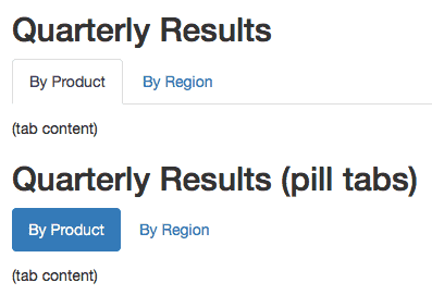
Tabbed Sections

One thing I found specially useful is the tabbed section. Tab layout helps to condense the parallel and lengthy content in the report.

Simply put {.tabset} tag after the markdown header and the sub-headers will become the tabs. The following code snippet gives an example

Tables, Data Summary & Plots

In Rmarkdown document, tables and plots are very common elements. I have a list of recommended packages to generate them in the document. In addition, I also found a data summary tools to produce a neat summary for data exploration and I always generate that in my appendix of EDA report.

• Tables: knitr::kable or DT::datatable
• Static Plots: ggplot2, ggpubr
• Interactive Plots: plotly, echarts4r, googleVis
• Data Summary: summarytools

The examples are demonstrated in the following embedded html document. The interactive plots are not properly rendered due to the incompatibility of my blog, however these should be perfectly working in the downloaded R markdown document. Again, the completed Rmd and rendered HTML report can be downloaded from here.

Rendering the document

There are some different options to render a html document from Rmd file.

1. For a notebook document: a nb.html file is automatically generated when the Rmd file is saved.
2. For a standalone R markdown document: click the blue knit button to render the html document.
3. For a separated R markdown document: add the one line of code (rmarkdown::render("input.Rmd", "html_document")) in R script to render the document.

Notes: The post is authorized to be republished here by Chaoran Liu, who is a very experienced data scientist working in Singapore. The original post can be found here.